3 R Basics
In this section, you will learn how to:
- Practice running code in the console window
- Perform basic arithmetic operations
- Create objects using the assignment operator
- Use functions to perform complex tasks
- Combine multiple operations
- Add a comment to a line of code
3.1 R as a calculator
You can think of R as a giant calculator. You type in a series of numbers and operators (+, -, /, *, etc.), press enter, and it evaluates what you typed and prints the output in the console.
Give it a try:
2 + 2#> [1] 4
4 - 1#> [1] 3
2 * 3#> [1] 6
7 / 3#> [1] 2.333333R uses standard MDAS order of precedence for operators: multiply, then divide, then add, then subtract. To change the order of operations you can use parentheses:
2 + 2 * 3#> [1] 8
(2 + 2) * 3#> [1] 12You can use exponentials like this:
3^2 # three squared is nine#> [1] 9Any text following a hash tag (pound sign) is ignored, which allows you to include comments in your code as seen above.
3.2 Assign values
Much like a human brain, R is not only capable of performing calculations, but also of remembering things, of storing them for later. This is accomplished using the assignment operator <- like this:
x <- 2Here we have told R to create space in its memory, store the number two there, and name that space “x”. Now, whenever we refer to x, R will know we mean 2.
Notice that the above code did not produce any output in the Console. After performing an assignment operation, you need to type the name of the object and press enter. Try printing x in the console:
x#> [1] 2You can now use x anywhere in your code, and R will always know what you mean:
x * 5#> [1] 103.3 The Environment tab
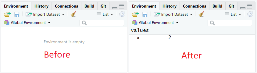
You may also have noticed that when you ran the assignment command, the Environment pane changed. Instead of saying “Environment is empty”, it now has a list of values, with one named “x”.
Try it again and watch how the environment changes:
y <- 7And you can use as many of these objects as you want in the same bit of code:
y / x#> [1] 3.5
z <- y + (x / 2)Try switching the Environment tab from List view to Grid view by clicking the word List.
To remove all the objects from the environment, you can click the broom button. If you switch to Grid view you can have the option of only removing the checked objects.
3.4 Functions
Some mathematical operations have no operator. For these you must use what is known as a function. For example, to take a square root:
sqrt(9)#> [1] 3A function consists of the name of the function followed by parentheses, with a list of arguments inside the parentheses. Some functions take one argument, some take more, and some take none at all.
A very commonly used function is c(), the combine function. This combines multiple values into what’s known as a vector:
k <- c(1, 2, 10, 4.7, 5.0)
k
#> [1] 1.0 2.0 10.0 4.7 5.0There are some functions that take vectors as arguments. For example, the the length() function returns the number of elements, or length, of a vector object.
length(k)#> [1] 5Useful mathematical functions include:
median(k) # median value#> [1] 4.7
mean(k) # mean value#> [1] 4.54
sd(k) # standard deviation#> [1] 3.501143You can even nest functions. In the example below, the c() function is evaluated first, and its value is used as the argument for the length function.
#> [1] 5Combining several of these features together, you can calculate the standard error of the mean (SEM) and a confidence interval around the mean for any set of numbers:
n <- length(k) # sample size
n
#> [1] 5#> [1] 1.565759Once you have calculated the SEM you can use it to estimate the upper and lower limits of a 95% confidence interval like this:
mean(k) + 1.96 * sem # upper limit#> [1] 7.608887
mean(k) - 1.96 * sem # lower limit#> [1] 1.471113#> [1] 7.608887 1.4711133.5 Self-assessment
Imagine you collected a sample of data which consisted of the following values:
6.05 4.89 3.32 4.93 5.25 5.04 4.91 2.84 5.60 5.34
Use the skills you have learned to answer the following questions:
- What is the sample size?
- What is the mean?
- What is the median?
- What is the standard deviation?
- What is the standard error of the mean?
- What is the 95% confidence interval? [two values]
Tip If you plan on using the same object names for the self assessment as you did for the tutorial (for example, k and n), it might be a good idea to clear your environment first. That way you won’t accidentally use the previous value of n (5) in your self assessment. To do this, click the broom icon in the Environment tab.
Once you are done, you can expand the section below to see the correct answers:
104.8174.9850.98997250.3130568-
5.430591 4.203409
Once you are satisfied with your answers, you can move on to the next activity.